

Parts List - Operations & Configuration
Configure parts, operations, production algorithms, cycle times, and downtime filters for accurate production tracking and analysis.
Overview
The Parts List is your central configuration hub for defining operations, parts, and production parameters. This page determines how IoTFlows tracks production, calculates cycle times, counts parts, and filters downtime events for each operation running on your machines.
Proper configuration in the Parts List is essential for accurate production tracking, goal setting, and performance analysis across the platform.
What is a Part/Operation?
In IoTFlows, a Part or Operation represents a specific manufacturing task or work order that produces units of output. Each operation has:
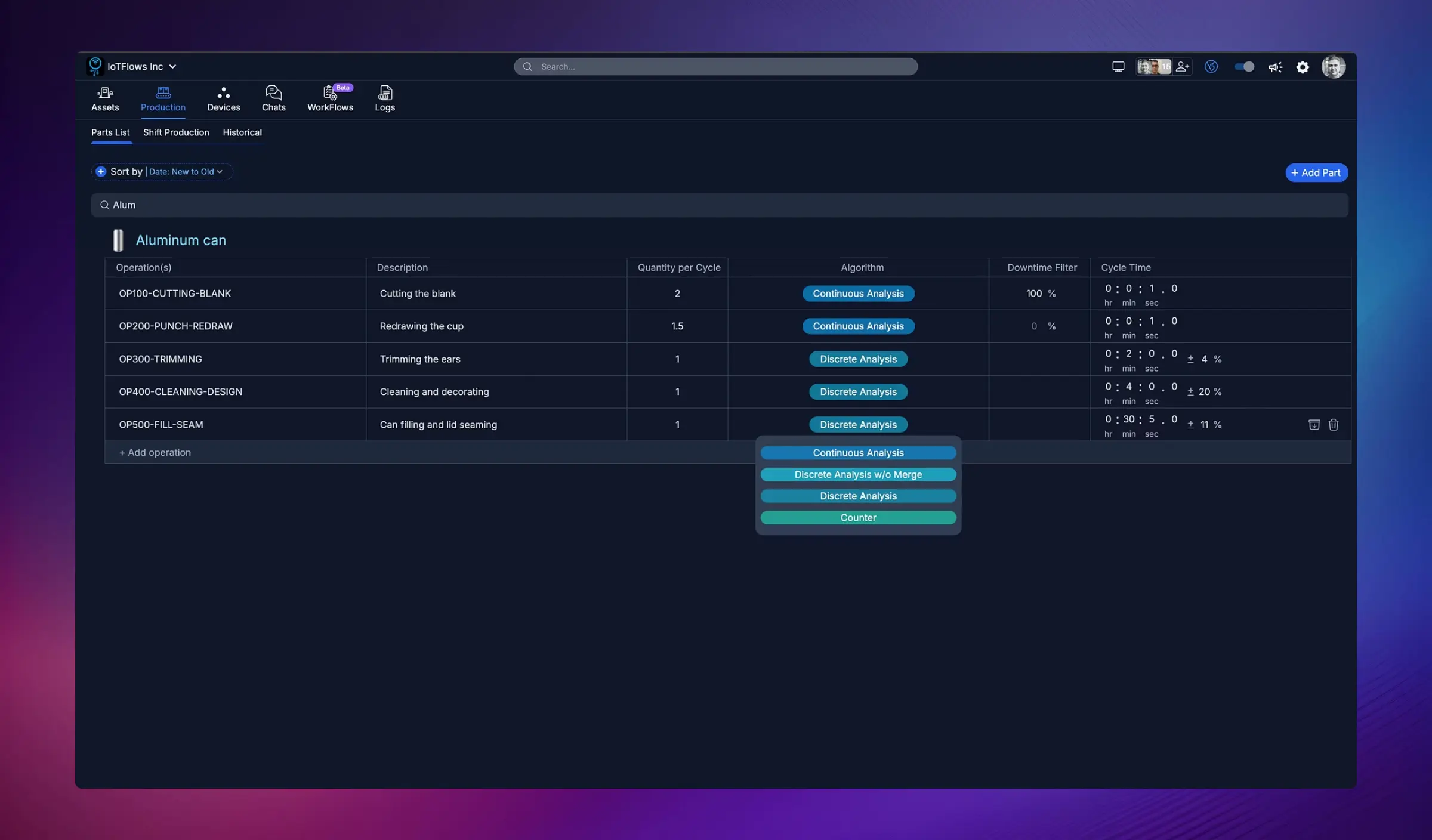
- Operation Name: Unique identifier (e.g., "OP100-CUTTING-BLANK", "OP30-GEAR-FINISHING")
- Description: What the operation does (e.g., "Cutting the blank", "Trimming the ears")
- Part/Material: What's being produced (e.g., "Aluminum can", "Bevel Gear 2")
- Quantity per Cycle: How many units produced per cycle
- Algorithm: How production is tracked (Continuous Analysis, Discrete Analysis, Counter)
- Cycle Time: Expected time per cycle or production rate
- Downtime Filter: Minimum downtime duration to ignore (optional)
Creating and Managing Operations
Add a New Operation
- Navigate to Production Tab → Parts List
- Click + Add Part in the top-right corner
- Search for the part/material (e.g., "Aluminum") or create a new one
- Fill in operation details:
- Operation Name (e.g., "OP200-PUNCH-REDRAW")
- Description (e.g., "Redrawing the cup")
- Quantity per Cycle (e.g., 1.5 if producing 1.5 cans per cycle)
- Select the Algorithm (see below for details)
- Set Cycle Time or Production Rate
- Optionally set a Downtime Filter percentage
- Click Save or Add Operation
Edit an Existing Operation
- Find the operation in the Parts List
- Click the edit icon (pencil) or click on the operation row
- Modify any field
- Click Save
Delete an Operation
- Select the operation
- Click the delete icon (trash can)
- Confirm deletion
Production Tracking Algorithms
IoTFlows offers four algorithms for tracking production, each suited to different manufacturing processes and sensor types:
1. Counter (BeamTracker Only)
Best for: BeamTracker laser-based counting systems
How it works:
- Counts discrete pulses from BeamTracker laser breaks
- Each pulse/beam break represents one or more parts (configurable with Quantity Per Cycle)
- Simple, direct counting with no pattern analysis
Cycle Time Usage: The cycle time you set defines the ideal or target cycle time used for:
- OEE calculation and performance tracking
- Production goal setting
- Calculating how many parts behind or ahead schedule
- Identifying when machines are running slower than expected
Use cases:
- Parts passing through a laser beam on conveyors
- Packaging lines with BeamTracker sensors
- Assembly lines with part detection
- Any operation using BeamTracker hardware
Example: A packaging line uses BeamTracker to count boxes. You set the ideal cycle time as 5 seconds per box. If boxes are passing every 6 seconds, the system calculates that you're running 20% slower than target.
2. Continuous Analysis (SenseAi/Embedded)
Best for: Continuous operations with known, consistent cycle times
How it works:
- Splits runtime by a specified cycle time
- Assumes production is continuous during uptime
- Converts small downtimes to uptime based on Downtime Filter percentage
- No cycle detection — purely time-based division
Cycle Time Usage: The cycle time you set determines:
- How many parts are counted (Runtime ÷ Cycle Time = Parts Produced)
- Example: 60 minutes runtime with 20-second cycle time = 180 parts
Downtime Filter for Continuous: The Downtime Filter percentage converts small downtimes back to uptime:
- Set as percentage of cycle time (e.g., 200%)
- Any downtime shorter than (Cycle Time × Filter %) is treated as uptime
- Example: 20-second cycle time with 200% filter → downtimes under 40 seconds become uptime
Best Practice: Injection Molding
Injection molding machines are perfect for Continuous Analysis:
Set accurate cycle time
Measure actual cycle time (e.g., 20 seconds per part)
Configure Downtime Filter
Set filter to 200% (or higher) to ignore brief pauses between cycles. With 20s cycle time, this converts downtimes under 40s to uptime.
Let it run
The algorithm splits runtime into 20-second intervals, counting one part per interval. Small pauses are ignored, giving accurate production counts.
Use cases:
- Injection molding machines (highly recommended)
- Stamping presses with consistent cycle times
- High-speed continuous operations
- Any process with predictable, repeating cycles
3. Discrete Analysis (SenseAi/Embedded)
Best for: CNC machines and operations with clear cycles and idle time between parts
How it works:
- Detects individual production cycles from vibration patterns
- Merges runtime and downtime to best match cycles within mean ± standard deviation range
- Counts actual detected cycles (not time-based division)
- Adapts to variable cycle times
Cycle Time Usage: The cycle time you set is used for:
- Goal calculations and OEE targets
- Comparing actual vs. expected performance
- Does NOT directly determine part count (actual detected cycles do)
How merging works:
- Analyzes patterns to find cycle boundaries
- Small pauses between cycles are merged into the cycle
- Longer stops are recognized as downtime
- Cycles must fall within statistical range (mean ± std dev)
Best Practice: CNC Machining
CNC machines often have small pauses (tool changes, repositioning) between parts:
Example: A CNC mill with 2-minute average cycle time:
- Discrete Analysis detects when each part completes
- Brief 10-second pauses for tool indexing are merged into the cycle
- Longer stops (operator intervention, maintenance) are captured as downtime
- Handles variation (some parts take 1:50, others take 2:10)
Use cases:
- CNC machining (lathes, mills, grinders)
- Manual or semi-automated operations
- Processes with variable but detectable cycles
- Operations with natural pauses between parts
4. Discrete Analysis w/o Merge (SenseAi/Embedded)
Best for: Machines with distinct picks, strokes, or impact events that should be counted individually
How it works:
- Detects actual vibration spikes/events without merging
- Each detected spike = one cycle counted
- Does NOT merge nearby events or small downtimes
- Counts raw detected events
Cycle Time Usage: The cycle time you set is used for:
- Goal calculations and targets
- Does NOT affect what gets counted (all spikes are counted)
Best Practice: Presses & Stroke-Based Machines
For machines generating distinct picks/strokes (e.g., punch presses, stamping machines):
Select Discrete w/o Merge algorithm
Choose this algorithm in Parts List for the operation
Set Downtime Filter on SenseAi device
Navigate to Devices Tab → Select the SenseAi sensor → Set Downtime Filter (e.g., 10 minutes)
How it works together
- Algorithm detects every pick/stroke as a cycle
- Device Downtime Filter converts all downtimes under 10 minutes to uptime
- Result: Perfect stroke counting with only meaningful downtimes captured
Example: A stamping press makes 60 strokes per minute:
- Discrete w/o Merge counts all 60 individual strokes
- SenseAi Downtime Filter set to 10 minutes removes micro-stops
- Only stops longer than 10 minutes are recorded as downtime
- Part count is accurate: 60 strokes/min × runtime minutes
Use cases:
- Stamping presses and punch presses
- Any machine with distinct picks/strokes
- Operations where every event should be counted
- Machines with high event frequency
Quantity Per Cycle
Quantity Per Cycle is a multiplier applied to all algorithms that adjusts how many parts each detected cycle represents.
How it works:
- Set as a number (can be fractional: 0.5, 1, 2, 6, etc.)
- Multiplies the detected cycle count by this number
- Works with ALL algorithms (Counter, Continuous, Discrete, Discrete w/o Merge)
When to use:
Multiple parts per cycle:
- Example: One machine cycle produces 6 identical parts simultaneously
- Set Quantity Per Cycle = 6
- Result: Each detected cycle counts as 6 parts
Fractional parts per cycle:
- Example: It takes 2 cycles to complete 1 finished part
- Set Quantity Per Cycle = 0.5
- Result: Two detected cycles count as 1 part
Most common:
- Set Quantity Per Cycle = 1 (one cycle = one part, the default for most operations)
Example: A dual-cavity injection mold produces 2 parts per shot. Set Quantity Per Cycle = 2. If the machine runs 100 cycles, you'll see 200 parts produced.
Cycle Time Configuration
Define expected production performance for each operation:
Option 1: Cycle Time (Time per Part)
Enter the expected time to produce one unit in HH:MM:SS format:
- Example 1:
00:02:00= 2 minutes per part - Example 2:
00:00:30= 30 seconds per part - Example 3:
00:00:00.5= 0.5 seconds per part (half a second)
Option 2: Production Rate (Parts per Minute)
Enter how many operations/parts should be produced per minute:
- Example 1:
120.0 ops/min= 2 parts per second - Example 2:
0.5 ops/min= 1 part every 2 minutes - Example 3:
90.0 ops/min= 1.5 parts per second
IoTFlows automatically converts between cycle time and production rate based on what you enter.
Downtime Filter
The Downtime Filter helps eliminate noise from very short, insignificant stoppages.
What it does:
- Ignores downtime events shorter than the specified percentage of cycle time
- Prevents micro-stoppages from cluttering downtime reports
- Focuses attention on meaningful downtime events
How to set: Enter a percentage (e.g., 100%, 20%, 4%):
- 100%: Ignore any downtime shorter than one full cycle time
- 20%: Ignore any downtime shorter than 20% of cycle time
- 4%: Ignore very brief stoppages (4% of cycle time)
Example:
- Cycle time: 2 minutes (120 seconds)
- Downtime filter: 20%
- Any stoppage under 24 seconds (20% of 120s) will be ignored
- Only stoppages ≥24 seconds will be recorded as downtime
Best practices:
- Start with 0% (no filter) to see all events
- Gradually increase the filter to remove noise
- For high-speed operations, use 1-5% to filter micro-stoppages
- For slower operations, use 10-20%
Algorithm Selection Guide
| Your Process | Recommended Algorithm | Device Type | Why |
|---|---|---|---|
| Conveyor counting / packaging | Counter | BeamTracker | Direct laser-based counting |
| Injection molding | Continuous | SenseAi/Embedded | Known cycle times with brief pauses |
| CNC machining | Discrete | SenseAi/Embedded | Variable cycles with natural idle time |
| Stamping presses / punch presses | Discrete w/o Merge | SenseAi/Embedded | Count every stroke, use device downtime filter |
| High-speed stamping (consistent) | Continuous | SenseAi/Embedded | Predictable cycle times |
| Manual assembly | Discrete | SenseAi/Embedded | Distinct work cycles with pauses |
| Low-volume custom machining | Discrete | SenseAi/Embedded | Variable cycle times with gaps |
Auto-Detect Operation
The Auto-Detect feature allows you to quickly configure which operation the platform should currently detect for a specific machine.
When to Use Auto-Detect
Use Auto-Detect whenever there's a setup change that requires detecting a new operation:
- Switching to a different part number
- Changing from one operation to another (e.g., OP10 to OP20)
- Starting a new job or work order
- After machine setup or changeover
How to Use Auto-Detect
Navigate to Assets Tab
Go to Assets Tab → Overview and locate the machine
Click on the machine
Open the machine's detail view
Click Auto-Detect button
Find and click the Auto-Detect button in the machine interface
Select the current operation
Choose which operation from your Parts List should now be detected for this machine
Confirm
The machine will now track production using the selected operation's algorithm, cycle time, and settings
Auto-Detect does not automatically know when you've changed operations. You (or the operator) must manually select the new operation whenever setup changes occur.
Best Practice: Operator Responsibility
Train operators to update Auto-Detect whenever they:
- Start a new job
- Switch part numbers
- Change operations after completing a run
This ensures production data is always associated with the correct operation and part.
Viewing and Sorting Operations
Search
Use the search bar to find operations by name or part description (e.g., search "Alum" to find all aluminum can operations).
Sort Options
Click Sort by and choose:
- Date: New to Old — Recently added operations first
- Date: Old to New — Oldest operations first
- Name (A to Z) — Alphabetical order
Add Operation Button
Click + Add Operation to quickly add a new operation to the list.
Best Practices
1. Set Accurate Cycle Times
Use historical data or engineering estimates to set realistic cycle times:
- Too aggressive → operators feel constantly behind
- Too conservative → no challenge or motivation
2. Choose the Right Algorithm
The algorithm significantly impacts data accuracy:
- Wrong algorithm → incorrect counts, misleading metrics
- Right algorithm → accurate production tracking and reliable analytics
3. Test and Refine
When configuring a new operation:
- Set initial parameters based on best estimates
- Run production for 1-2 shifts
- Review actual vs. expected counts
- Adjust algorithm, cycle time, or downtime filter as needed
4. Use Descriptive Names
Operation names should be clear and consistent:
- Good: "OP100-CUTTING-BLANK", "OP200-PUNCH-REDRAW"
- Bad: "Op1", "Process A", "Machine 5 Job"
5. Document Operation Details
Use the Description field to add context:
- What the operation produces
- Special setup notes
- Quality checkpoints
- Material specifications
Common Issues and Solutions
Production Count is Too High
Possible causes:
- Algorithm counting noise or vibrations as parts
- Cycle time set too short
- Downtime filter too low
Solutions:
- Switch to Discrete Analysis if using Continuous
- Increase downtime filter percentage
- Verify sensor isn't detecting non-production events
Production Count is Too Low
Possible causes:
- Algorithm missing actual production cycles
- Sensor misaligned or not detecting properly
- Downtime filter too aggressive
Solutions:
- Switch to Continuous Analysis if using Discrete
- Reduce downtime filter percentage
- Check sensor placement and calibration
- Verify machine is actually producing at expected rate
Cycle Time Doesn't Match Reality
Possible causes:
- Incorrect algorithm selection
- Machine running slower/faster than expected
- Multiple operations merged into one
Solutions:
- Review actual production data over several shifts
- Adjust cycle time to match observed reality
- Split into multiple operations if needed
Need help configuring operations or choosing the right algorithm? Contact our support team at support@iotflows.com